Stabilising Small World Models With Flow Forcing

Open Table of contents

Introduction
Model
Data
Training
Inference
Results
- Failure modes
Next steps

Introduction

There are a lot of arguments online about whether LLMs develop implicit world models as an emergent property of next-token-prediction objective based training.

However, I’m very interested in models which are designed as explicit world models. More concretely, they model the following probability $p(s_t\mid s_{1: t-1}, a_{1: t})$ , Where $s_t$ and $a_t$ are the state and action at time $t$ . The coolest examples of these are generated gameworlds which allow for realtime interaction, like Decart’s OASIS model, where you can play a game in a purely generated environment that is created on-the-fly. Wayve’s GAIA 1 and GAIA 2 models are also good examples of these types of models, which can generate interactive and controllable driving scenarios.

Example of OASIS model generating interactive gameplay. Source

Questions about long term consistency aside, there is an issue with training these types of model with the traditional “teacher-forcing” objective commonly seen used to pretrain language models. “teacher forcing” roughly means obtaining a ground truth partial trajectory $s_{1:t-1}, a_{1:t}$ and attempting to learn a parameterised distribution over the next state using some loss between the model’s prediction and the ground truth next state.

However, one thing autoregressive diffusion/flow matching models built in this way suffer from is compounding errors. That is, because the model is only trained on predicting the next state from ‘perfect’ historical trajectories, the inference setup of autoregressive rollout results in little errors which accumulate and push the trajectory further and further away from the distribution that the model has become accustomed to seeing in training. Ultimately, this results in trajectories which are unstable and degrade very quickly.

One way of looking at this error is as noise added to the new state, which corrupts it. What if we could model this inference-added noise which isn’t taken into account during training? A paper called Diffusion Forcing: Next-token Prediction Meets Full-Sequence Diffusion takes this idea and cleverly changes the standard teacher forcing objective into one that accommodates for this noise, which I’ll refer to as flow forcing. The paper goes into more detail, but the high level idea is that a single sequence of $N$ states acts as $N$ training subexamples, where each state is noised independently, and we compute the standard flow matching objective for each frame. Critically, the model gets the noised history of previous states, with the strength of the noise that has been applied at each state. This allows the model to selectively grab information from past states with the knowledge that some past states are more information rich than others.

Read the paper for implications and the different modes of operation this setup can facilitate, but ultimately this allows for robust autoregressive rollout, since, during the rollout, we can noise previously generated frames on purpose and tell the model we have noised them, so that we can “cover up” the weakness of the model and focus on the information that it can glean across the sequence of frames, rather than strongly relying on most recent state for prediction (which is a good strategy if the state is clean/well generated).

The following is an attempt to try testing this idea by creating a small driving simulator.

Model

The model architecture isn’t super interesting; if you understand the autoregressive transformer model, you’ll probably understand diffusion/flow matching transformer models.

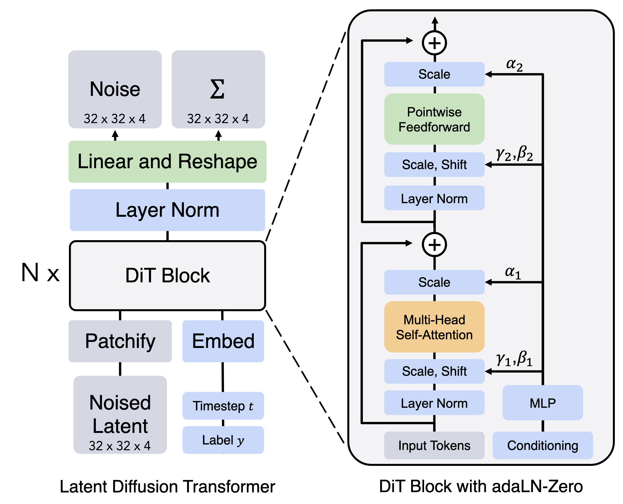
The “diff” between a standard transformer and my model is as follows:

Tokenization and Detokenization: To feed our input into the model, we need to convert a sequence of frames with overall shape $[T\;H\;W\;C]$ into $[S \;d_{model}]$ . One naive way to do this would be to flatten the $T,H,W$ dimensions into a rasterisation style manner, then project the $C$ dimensional vector into $d_{model}$ . However, this would result in an effective sequence length of $THW$ , which would be too big to effectively model (a 4s 10fps clip at 480x768 would be 15M tokens per sequence!). There are two ways to reduce this:
- Patchifying: Patchifying the input into e.g 4 x 4 squares of pixels, flattening into a 443 dimensional vector and projecting this up into $d_{model}$ . This reduces the sequence length by a factor of $f^2$ . Increasing this too far can be problematic since you might enter a situation where each token covers too big a receptive field.
- Modelling in latent space: We can reduce the spatial dimensions of the image by using an autoencoder and performing flow matching in latent space. In the above explanation, C would be 3 (RGB channels). However, these autoencoders output “images” with 64x fewer “pixels” (where each image dimension has reduced in size by a factor of 8) but each “pixel” is semantically richer, with 16 channels rather than 3. In practice, I applied both of these techniques.
- LocalViT style depthwise convolution: With small models, I sometimes found it was useful to add depthwise convolutions in the up projection of the MLP layers to mix information from neighbouring tokens, rather than relying solely on attention (LocalViT). I’m not sure this is necessary at bigger model sizes though, but it is relatively inexpensive to compute so I kept it.
3D position embeddings: By default, most modern transformers use 1D rope embeddings to tell the model the position of tokens in the sequence, which makes sense for 1D sequences like language. However, using this for our setup means that the model has to learn the mapping between t, x, y dimensions and the 1D rasterisation during training. Therefore, I used spatiotemporal 3D RoPE so the model doesn’t have to learn this so implicitly, though I haven’t ablated so maybe it doesn’t matter too much.
Sliding chunkwise attention: Traditional attention is quadratic in complexity, since each token has to attend to all previous tokens. Sliding window attention is one common method for getting around this, by restricting the number of tokens the model can see to the N previous tokens, where N is the size of the window. In our model, we implement the sliding window at the frame level rather than at the token level, since one entire frame is modified every forward pass, rather than generation of a single token. This means that every token can attend to each token in the same frame, but also to all tokens in the previous N frames. This can be efficiently implemented in Flex Attention.

Worth noting that although the model trained uses 10 frames (i.e 1 second) of history in the attention, the current frame can see further back than this, since we stack multiple layers, which allows composition of high level features (like the colour of a car 20 seconds ago that’s been out of frame for a while) over larger timescales.

I did also implement group query attention as it was fairly easy to, but as I understand this is mostly an inference time optimisation to reduce the size of the KV cache, so wasn’t super important for me and I left it off.

My final model had 36 layers, 4 attention heads per layer, $d_{model} = 1536$ , with 2.4B parameters.

Data

The training data predominantly comes from the vista dataset, which consists of high quality driving 4k driving videos which I downloaded, downsampled to 480p 10fps and cut up into 4s clips. Together with 14422 clips applying the same process to the nexar dashcam accident dataset, which has per second time of accident labels which I applied as conditioning labels into the model, we arrive at a total of roughly 850k 4 second clips. For my main model, I found that it seemed to converge having seen 270k clips, so stopped training here to save on compute costs.

Training

Objective

This blog is definitely not supposed to be a guide for how diffusion/flow matching works. I recommend this paper for a comprehensive guide to flow matching. However, the algorithm is relatively straightforward, and is shown below: It ends up boiling down to per frame noising of the input coupled with the flow matching objective summed across each frame in the sequence.

Algorithm: Flow Forcing Training

\begin{gathered} \begin{aligned} &\textbf{Input:} \text{ Video sequences } x_{1:T} = \{x_1, x_2, \ldots, x_T\}, \text{ accident flags sequences } a_{1:T} = \{a_1, a_2, \ldots, a_T\} \\ &\textbf{Output:} \text{ Model parameters } \theta \\ \\ &\textbf{for } \text{each training iteration } \textbf{do} \\ &\quad \text{Sample batch of video sequences } \{x_{1:T}^{(i)}\}_{i=1}^B \text{ with flags } \{a_{1:T}^{(i)}\}_{i=1}^B \\ \\ &\quad \text{// Sample independent timesteps and noise for each frame} \\ &\quad \tau_{1:T} \sim \text{Uniform}(0, 1)^T \text{ (independent for each frame)} \\ &\quad \epsilon_{1:T} \sim \mathcal{N}(0, I)^T \text{ (independent for each frame)} \\ &\quad \tilde{x}_{1:T} = \tau_{1:T} \odot x_{1:T} + (1 - \tau_{1:T}) \odot \epsilon_{1:T} \\ &\quad \text{where } \odot \text{ denotes element-wise multiplication} \\ \\ &\quad \text{// Forward pass on noisy sequence} \\ &\quad v_\theta(\tilde{x}_{1:T}, a_{1:T}, \tau_{1:T}) \leftarrow \text{FlowTransformer}(\tilde{x}_{1:T}, a_{1:T}, \tau_{1:T}) \\ \\ &\quad \text{// Compute flow matching loss} \\ &\quad v_{\text{target}} = x_{1:T} - \epsilon_{1:T} \\ &\quad \mathcal{L} = \frac{1}{|\mathcal{M}|} \sum_{t \in \mathcal{M}} \|v_\theta(\tilde{x}_t, a_t, \tau_t) - (x_t - \epsilon_t)\|_2^2 \\ &\quad \text{where } \mathcal{M} \text{ is the set of masked (valid) frames} \\ \\ &\quad \text{Update } \theta \text{ using gradient descent on } \mathcal{L} \end{aligned} \end{gathered}

Liger Kernels

One simple way to speed up training is to use torch.compile. I also used the custom Triton kernels provided by the Liger library, for things like RMSNorm and SwiGLU. I think speed benefits from using these are most apparent during multi-GPU training, so perhaps this is something worth ablating on my single-GPU setup.

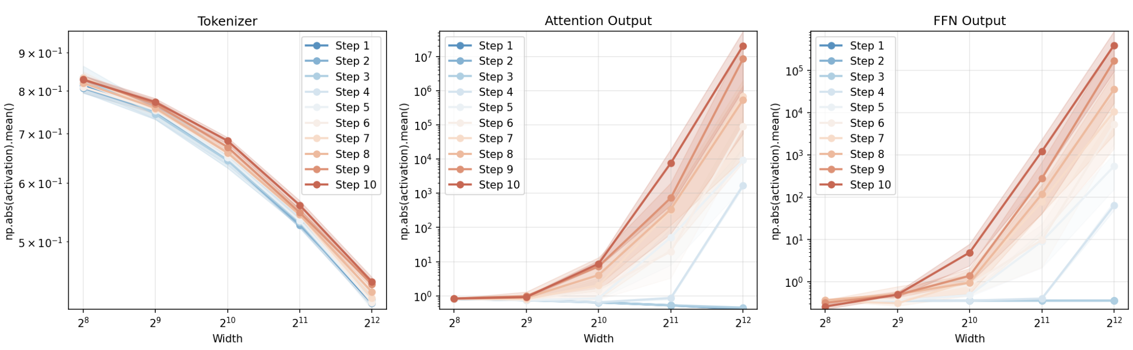
MuP initialisation

When training a really big model, often you can’t afford to do a big sweep over hyperparameters to work out the best set for that specific setup. Ideally, what you want to be able to do is find optimal settings for things like learning rate, init std for weights using a smaller model, then transfer these to the bigger setup. However, this tends not to work if you do it naively; the best learning rate changes with model scale. However, there is a specific way of scaling these parameters with model size, called Maximal Update Parametrization, which allows this transfer. I implemented this, and the training across a few steps looks more stable across model width with MuP:

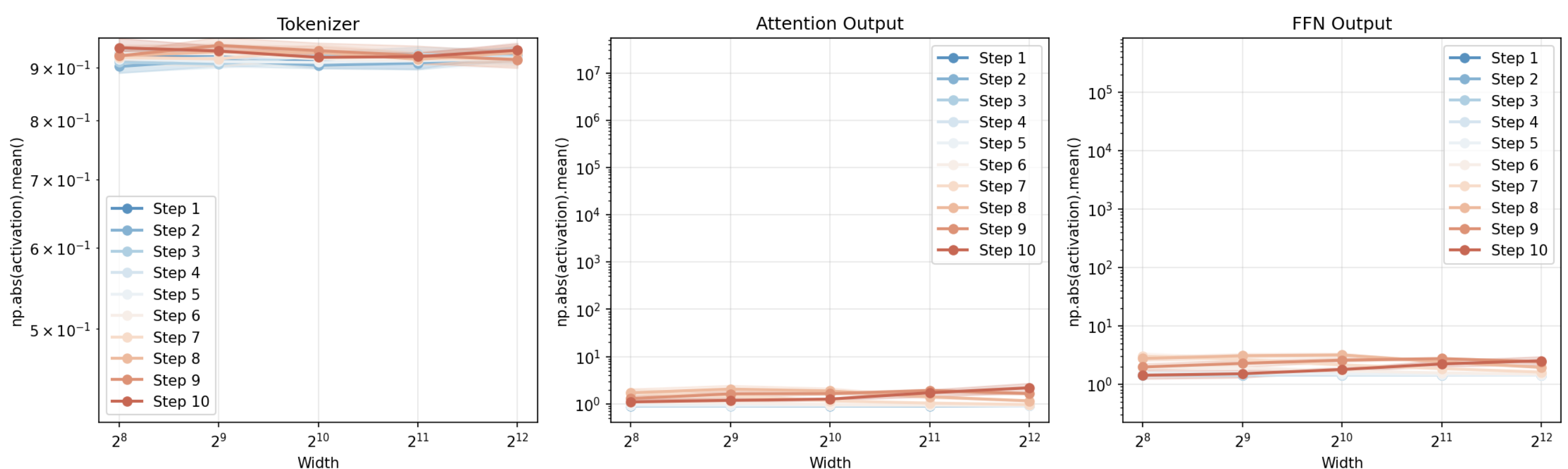
Training loss without MuP initialization — Activation sizes across width with MuP off

Training loss with MuP initialization — Activation sizes across width with MuP on

I did however end up turning off the scaling of the final readout/detokenizer layer and extra $\sqrt{d_{head}}$ scaling on $QK^T$ , since I found this bottlenecked performance. I suspect the problem is more with the detokenizer scaling - if the output of the model is scaled down too much, it might prevent the output being of the right scale as compared to the ground truth, meaning the weights have to be very large to compensate, which is quite challenging to achieve if you use weight decay which opposes this. The softmax over vocab in a traditional LM makes this a nonissue as it normalises.

The optimal setting for hyperparameters was obtained with Bayesopt on a model 10x smaller than the final one. I also used a relatively small batch size of 4 for the final training run, since in a single GPU setup where small batch sizes can be decently efficient in terms of MFU, gradient accumulation is not useful (see here) for more details. I also had to use gradient checkpointing on the attention computations to fit the model in memory.

One gotcha with MuP is that it allows you to transfer HPs given a fixed data budget; if you also scale up the amount of data you use along with model size, there is no guarantee that your optimal hyperparameter setup is still optimal! Ideally what you would do is do a multiobjective hyperparameter optimisation for minimising flops and loss for a fixed model size but optimising both the HPs and dataset size and fit scaling laws, but I was cheap and ended up fudging it based on advice from this great blog post.

Inference

To perform a stable rollout with the trained model where divergence is an issue we have two options:

Do a standard for loop to generate new frames, but tell the model that the previous frames generated are noisier than they should be, by setting the $\tau$ flow matching timestep to be less than 1, where 1 implies a clean frame.
Same as above, but maintain a separate cache history of noisy frames that are the “clean” generated frames that are then noised on purpose, and condition the model with the frames with the appropriate $\tau$ according to the noise level used.

Since the “noise” from the model being bad is not likely to be Gaussian, I chose the latter option as it seemed more principled. Here is a proper explanation of how this works:

Algorithm: Stable Autoregressive Rollouts

\begin{gathered} \begin{aligned} &\mathbf{Input:}\ \mathrm{Initial\ frame\ } x_1,\ \mathrm{total\ frames\ } T,\ \mathrm{regularisation\ strength\ } \alpha \\ &\mathbf{Output:}\ \mathrm{Generated\ video\ frames\ } \{x_t\}_{t=1}^T \\ \\ &\mathcal{C} \leftarrow [x_1] \quad \mathrm{//\ Clean\ frames} \\ &\mathcal{N} \leftarrow [x_1] \quad \mathrm{//\ Noisy\ context\ frames} \\ \\ &\mathbf{for\ } t = 2\ \mathbf{to\ } T\ \mathbf{do} \\ &\quad \mathrm{//\ Prepare\ regularized\ context} \\ &\quad \tilde{x}_{\mathrm{context}} \leftarrow \mathcal{N}\ \mathrm{with\ noise\ levels:} \\ &\qquad \tau_1 = 1\ \mathrm{(first\ frame\ stays\ clean)} \\ &\qquad \tau_i = 1 - \alpha\ \mathrm{for\ } i > 1\ \mathrm{(regularisation\ noise)} \\ \\ &\quad \mathrm{//\ Generate\ clean\ frame\ using\ flow\ matching} \\ &\quad x_t \leftarrow \mathrm{Denoise}(\tilde{x}_{\mathrm{context}},\ \mathrm{position}=t) \\ &\quad \mathrm{where\ Denoise\ integrates\ from\ } \tau=0\ \mathrm{to\ } \tau=1 \\ \\ &\quad \mathrm{//\ Update\ caches} \\ &\quad \mathcal{C} \leftarrow \mathcal{C} \cup \{x_t\} \\ &\quad \tilde{x}_t \leftarrow (1 - \alpha) \cdot x_t + \alpha \cdot \epsilon, \quad \epsilon \sim \mathcal{N}(0, I) \\ &\quad \mathcal{N} \leftarrow \mathcal{N} \cup \{\tilde{x}_t\} \\ \\ &\mathbf{return\ } \mathcal{C} \end{aligned} \end{gathered}

Results

In each clip, the model receives the same (high quality) starting image, and performs an autoregressive rollout a series of 29 new frames, which results in a three second clip. From left to right, the regularisation level increases (the levels used are $[0.0,0.1,0.2,0.3,0.4]$ ).

Very qualitatively, I noticed slightly better consistency as the regularisation was increased, but this was not perfect in all cases. For example, in the following clip, the motion of the signpost looks better with higher regularisation, but the left car seems to smear more rather than being passed by as is the case with low regularisation.

Movement of signposts is correct

I particularly like the following example, where the direction of travel of the other car changes in different rollouts:

Car drives in opposite directions on different rollouts

Overall, perhaps unsurprisingly, the model does best in very simple scenes, where the benefit of the regularisation is somewhat clearer:

Example of Autoregressive Rollout

If you really squint at the low regularisation examples, it kinda looks like the right car is overtaking the left one here (but perhaps I’m reaching too much).

Example of overtaking?

Failure modes

I did notice a number of failure modes with the rollouts, regardless of how much regularisation was used.

Firstly, approaching a car in front from behind can cause instability, and the model stretches it out in an non-physical way past a certain point in the trajectory. You do get a good sense of motion in the periphery though.

relative motorcycle speed changes in different rollouts

Secondly, the model does not deal with turns well at all. I guess turns are much less represented in the training data than long stretches of straight driving, but the model really likes to drive “forward”, often inventing/shifting the direction of the road to make this more feasible.

Light turning causes issues

Model can't deal with sharp right turns

Another poor turn

I’m not going to pretend this is a particularly good world model, but for just under £200 (very roughly 100x less than the world model pretraining costs of GAIA-1) I don’t feel too bad about the quality of the samples that I ended up with.

Next steps

That said, I think there are a bunch of things that I’d like to try out next:

Improved training efficiency: After all my attempts at optimising the training of this model, I ended up with an MFU of… 7% 😬. I think this is quite bad, particularly for a single GPU setup where there is no extra overhead with distributed training. I need to investigate whether this is caused by a bottleneck in streaming data in with the library I’m using (MosaicML’s streaming dataset library), or some other issue.
Scaling Laws: Although I don’t think the quality of the rollouts is fantastic, I’d really like to establish a proper Flop/FVD scaling law, so that I could say “given 100x more compute budget, I could achieve the same quality as a leading open source generative world model”. Secondarily, I think that as models get better at modelling the next state, the train/test problem goes away somewhat, so you may get more value from your data by training in a teacher forcing way rather than on noise masks that you never end up seeing during inference.

Attempting to hyperoptimise FLOP/dollar by using a single discounted GH200 lambdalabs instance to pretrain a 2.4B model.
Improved inference efficiency: Sampling a rollout is very inefficient at the moment. In a rollout given above, we get 120 spf (N.B not fps!) with a single A100. I implemented sampling in the most naive way possible with zero optimisation, so there are a number of things to improve this:
- The first one is adding a KV cache, since we unnecessarily recompute them for previous frames when we don’t need to.
- Secondly, I use 100 flow matching steps per frame; if I could get good results leveraging the methods from few step flow matching models, like MeanFlow, a speedup of 100x could be on the cards.
- It’s also typically grossly inefficient to sample an autoregressive transformer model at batch size 1, and in this regime, you are usually heavily memory bandwidth bottlenecked, rather than compute bottlenecked. I’m not sure this strictly applies here, since, unlike a standard LLM where you generate one token at a time, with this model you have to do a full forward pass across all tokens that make up a frame in the video. That being said, I did see some interesting work by the Alibaba group on leveraging multiple parallel forward passes on the same input with slightly different augmentations to leverage more computation where memory bandwidth can be bottlenecking.
Interactivity: At the moment, this is a pretty weak example of a world model, since the only interactivity that can influence the future states rolled out by the model is the accident flag. I haven’t shown any results with this flag enabled, but I imagine the quality of the model would prevent me from getting interesting results at the moment. An interesting question is whether it’s better to use the limited amount of data I have for this during pretraining or a separate fine-tuning stage (intuition is probably the latter is better).
Architectural comparisons: I find it interesting that GAIA-I and GAIA-II switched from a vanilla autoregressive transformer operating over VQVAE based image tokens to a flow matching transformer similar to the setup presented here. I don’t have strong intuitions here - I might have assumed that inference from the AR discrete token transformer would be faster, but I guess it depends heavily on how many flow matching steps you can get away with in the second setup. There’s probably an opportunity to test out architecture specific modifications here too, like MoE or alternative global/local sliding window attention.
Model predictive control with world models: This model is far too weak and slow to facilitate this; however, one alternative to policies that that just model $p(a_t | s_{1:t-1}, a_{1:t-1})$ is to perform model predictive control using the world model. This would look like optimising a sequence of actions based on one or multiple possible futures, taking the first action in the sequence, then throwing out the rest of the sequence and doing the whole thing again at the next timestep. Perhaps standard learned policies already do this implicitly, but could still be an interesting avenue (if you can make the world model very fast & on device!).
Driving policy auditing with world modelling: Thinking further out, I think these types of models offer an interesting type of auditing opportunity for the growing number of companies that offer self driving - you could have a standard world model shared across the industry which simulates consistent and reproducible driving scenarios for a third party to test different providers’ approaches against.